How to link Sheets or Tabs in Excel to a master sheet

Excel offers ample flexibility for a wide range of tasks. We just need to know the tools, functions, and options it has. The rest is easy. One of Excel’s features is the ability to link sheets, tabs, cells, tables, etc., across other sheets, making data analysis and access easier. It is like creating a table of contents for Excel and its data. In this guide, we show you how to link Sheets or tabs in Excel to a master sheet.

How to link Sheets or Tabs in Excel to a master sheet

Learn all about linking sheets, tabs, individual cells, a range, or a table, and more in the following ways.

Link Sheets to a Master Sheet
Set up automatic updates or calculations

Let’s get into the details and see how we can improve Excel usage with linking.

Link Sheets to a Master Sheet

We can create a master sheet in a Workbook and link other sheets to it, and create links to access them instantly. This gives us a lot of convenience in managing data and multiple sheets. It makes it easy to manage sheets by categorization or the essence of the sheets.

Open an Excel workbook and create some sheets. We have created a few sheets. Named the main sheet as Master Sheet.

Now, we link Sheet 1 to Sheet 10 to the Master Sheet. Create a Table in the Master Sheet. It should have a serial number, the name of the sheets, and a link. After creating, click Insert on the ribbon menu and select Table. Ensure you check the button beside My table has headers on the Create Table pop-up. Then, click OK.

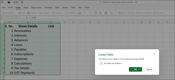
Now, we need to link the sheets via a hyperlink on the C column. Click the C2 cell and paste the following formula.

=HYPERLINK("#'" & [@[Sheet Details]] & "'!A1","Open")

You can replace Open in the formula with any text you like.

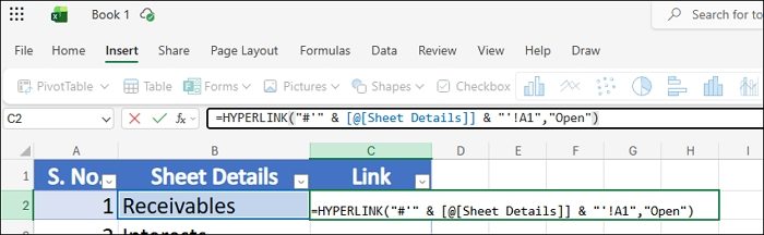
The links will apply automatically to every cell in the C column as the table is structured. If you add a new sheet in the future, just add another row at the bottom of the table and enter the new sheet name in column B. The formula will autofill and apply in the C column for the new sheet.

Set up automatic updates or calculations in Excel

Now, if we want to see a calculation directly from any of the sheets, we can do so in two ways. One is by linking directly to the calculated cell in the particular sheet, or dynamically using the INDIRECT function.

The first method is to link to the cell directly. If you want to see the total amount from a sheet directly on the Master Sheet, you have to first calculate the sum of all the entries in the sheet using the SUM function. Then, in the master sheet, type = and then click on the sheet you want to get the data from and select the cell there. After the correct selection, it should look like the following image. The column or row might change based on your preference.

The cell you have selected to link on the master sheet must not be changed to another cell. If you change it, the pulled data may be incorrect. You have to update it when you change the SUM function of the sheets to another cell.

If every sheet has the same cell to link to the master sheet, you can use the INDIRECT function. For example, if you want to see the cell data from B10 on every sheet on the master sheet, you can use the following formula.

=INDIRECT("'" & B2 & "'!B10")

Replace B10 with whichever cell you want to pull. The formula will apply to all the cells below on the master sheet if you apply on the structured table.

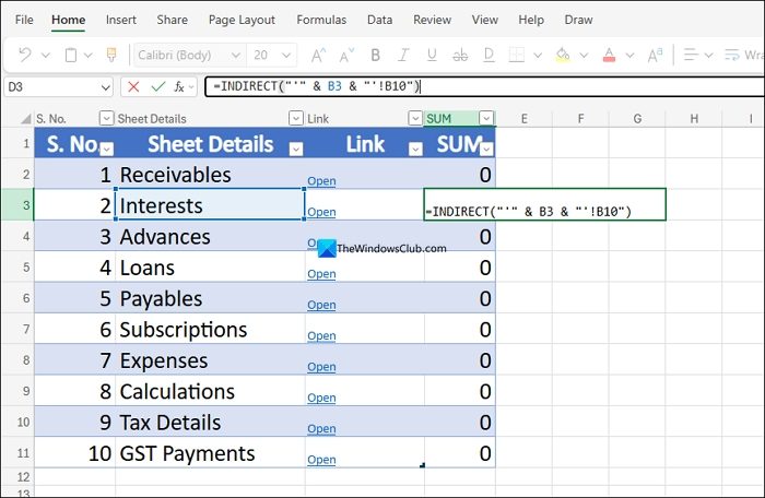
Remember that it pulls the same cell from all the sheets. If the sheets have different cells, you need to pull the data into the master sheet, then use the direct method.

Read: How to connect Google Sheets with Excel

How do I link all sheets to one sheet in Excel?

To link all sheets into one sheet in Excel, create a new sheet as the Master Sheet, then connect them using the Hyperlink function. You can just create a dashboard with just hyperlink, sum, indirect, and direct linking methods in Excel.

How to make a link to a specific sheet in Excel?

To create a link to a specific sheet in Excel, open the sheet you want to link to. Then, type =HYPERLINK(“# and select the sheet and its first cell, type a “ and comma, and enter the name for the link with double quotations, and close the formula with ). It should look like the following.