Have you ever tracked your income and expenses and had a realistic approach towards personal finance? It takes a lot of discipline to understand and plan your family’s budget. Without a clear budget, it will be a war with finances at the end of each month. You can neither remember the expenses you made, nor how much you are spending on each necessity of yours. If you are struggling to keep up with your budget and want to track and automate your budget on Excel for free, this guide is for you. We show you how to create a budget or personal finance dashboard to keep your expenses in sync with reality.
What do I need to automate my budget in Excel?
To automate your budget in Excel, you need an Outlook account to create and use Excel. Then, you must have a list of your income sources, an expenses list, and other information related to your personal finances that helps in creating a realistic budget in Excel.
How to create an automated Budget in Excel
To automate and track the budget in Excel, we need clear data on income and expenses by category (e.g., groceries, housing), and a clear dashboard from the data you input. We will focus on these and create a personal finance workbook in Excel.
- Create three sheets
- Record every transaction in the right columns
- Setup categories
- Automate the summary of finances
- Get insights into the total budget with Net Income
Let’s get into the details and create a workbook in Excel that you can use every month for your budget.
Open Excel on your PC and create a new Workbook. Name it “Monthly Budget” or whatever you feel suits it. Sheet1 is created by default in the Workbook. Right-click on it and rename it as “Income & Expenses.” Now, click the + icon beside it to create a new sheet. Rename this as “Categories.” Create another sheet and name it “Dashboard“.
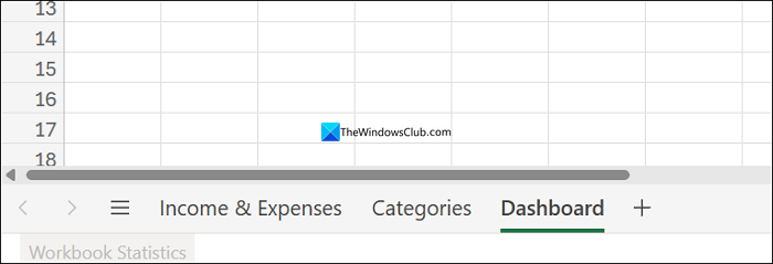
As the names suggest, we must record all income and expenses in the Income & Expenses tab; the Categories tab contains different categories of expenses and income; and the dashboard shows the report based on the other two sheets.
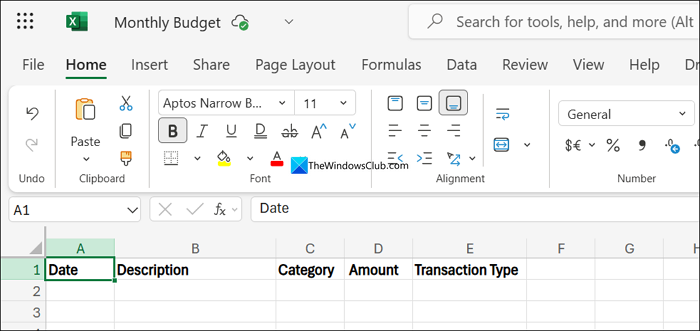
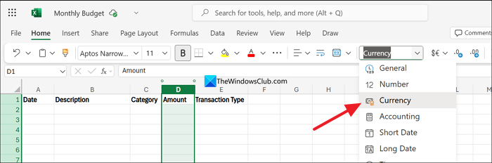
Now, set up the Income & Expenses sheet to record all the transactions to get a clear picture. Click on the Income & Expenses sheet and create the Date, Description, Category, Amount, and Transaction Type columns, as shown in the image below.
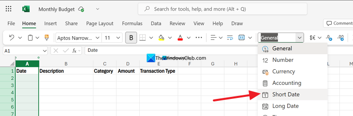
After creating the columns, we need to format them accordingly. To do that, select the entire A column by clicking on it. When the A column is highlighted, click on Home in the ribbon menu. Then, on the number tab, click the General drop-down menu and select Short Date.
Then, set the Amount format by clicking on the D column. Then, click the drop-down button in the number tab and select Currency.
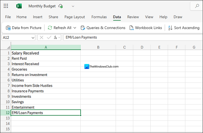
Now, click the Categories sheet. In this sheet, we define various categories in Income and expenditure. To get the right outlook on finances, we need to be consistent with spelling. Even if we miss a letter, Excel treats it as a new category and messes up the entire Workbook. Keep it in mind while entering the values in the Income & Expenses sheet.
List out all the income and expenses categories you normally receive or spend money on in a single column, as shown in the image below.
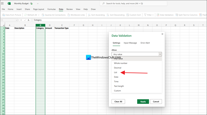
Now, we need to connect these categories to the Category column on the Income & Expenses sheet using Data Validation options. Click on the Income & Expenses sheet, and select the entire Category column. After selecting it, click on Data in the ribbon menu and select Data Validation in its options. It will open a Data Validation pop-up. Click the Allow drop-down and select List from the options.
You need to select a source for the list. To do that, click the Categories sheet and select the cells where you have entered all the possible income and expenses categories. Then, click Apply to save it.
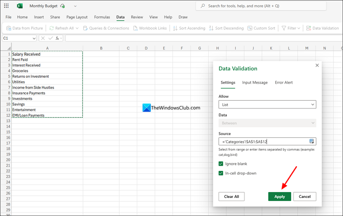
You will now see a drop-down button beside every cell in the Category column on the Income & Expenses sheet. It is now time for the automation of all these income and expenses to see a picture of your finances.
Click the Dashboard sheet and create a table with Category, Budget Allocated, Actual Received/Spending, and Difference. In the Category column, fill each category with the categories you have listed earlier in the Categories sheet. Then, fill the Budget Allocated column with your estimates.
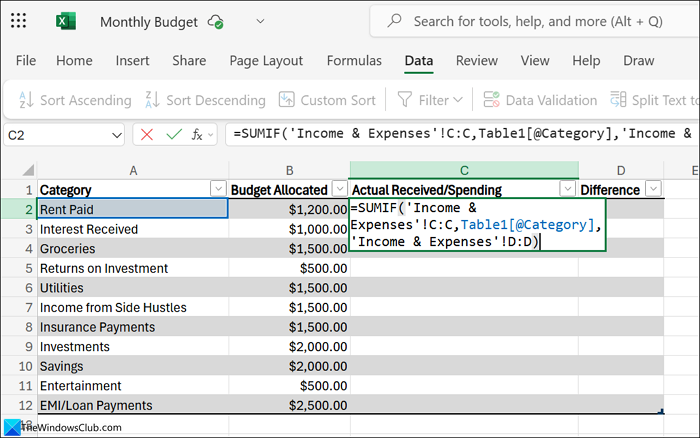
To automate the actual spending column in the Dashboard sheet, we will use the SUMIF function. It may look too complicated, but follow our instructions carefully.
SUMIF function syntax contains three elements. The first one is range. Range defines where to look. The second one is the criteria. It can be looked at as a rule. Criteria can be termed as a category, like Rent paid, groceries, etc. The third element is the range, in this context. A comma separates each element, and brackets enclose all three elements together.
To put it simply, the first and third elements in the syntax are from the Income & Expenses sheet. The second element, or criterion, is in the Dashboard. Let’s write the syntax to calculate the total amount spent on a category, such as Rent paid.
We are calculating the amount spent on rent. So, go to the cell related to Rent Paid under Amount Received/Spending. Then, type =SUMIF(. Now, select the first element, which is the Category column in the Income & Expenses sheet. Click the Income & Expenses sheet and click column C to set it as a range. Shift to the Dashboard sheet and type , (comma) to enter the second element. The second element is the Rent Paid cell in the Dashboard sheet. In the image below, it is A2. So, select A2 cell followed by a comma. Then, head to the Income & Expenses sheet and click the D column to select the Amount column as the third element in the function.
=SUMIF('Income & Expenses'!C:C,A2,'Income & Expenses'!D:D)
Drag the SUMIF function to apply it to every other category. Now, we need to calculate the Difference between the allocated budget and the actual amount spent or received. To calculate that, go to the Difference column and select the first cell. Type = and select the Budget allocated cell in the same row, type a minus, and then select Actual Received/Spending amount in the same row and press Enter.
= B2 - C2
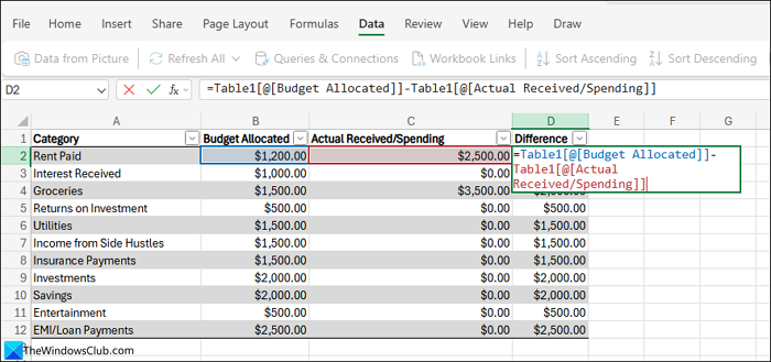
Drag and apply the same formula to the remaining categories.
Now, we need to calculate Net Income, which is Total Income subtracted by Total Expenses.
Net Income = Total Income – Total Expenses
We will again use the SUMIF function to calculate Net Income. It involves calculating Total Income using the SUMIF function, then Total expenses using the SUMIF function, and then Net income with the subtraction formula.
To calculate Total Income with the SUMIF function, use the following Syntax. Use it below the table on the Dashboard sheet.
=SUMIF('Income & Expenses'!E:E, Income, 'Income & Expenses'!D:D)
To calculate Total Expenses with the SUMIF function, use the following Syntax.
=SUMIF('Income & Expenses'!E:E, Expenses, 'Income & Expenses'!D:D)
Now, to calculate Net Income, subtract Total Expenses from Total Income on the sheet.
Also read: Free Personal Finance & Business Accounting Software for Windows PC
Can I use Excel to make a budget?
Yes, Excel has many powerful formulas and functions that can help you create a budget that works for you, based on your income and lifestyle. You need to understand the syntax of each function and apply it carefully. It has a steep learning curve, but once you understand it, there will be no stopping you from budgeting in Excel.
Related read: How to use COPILOT in Excel.