How to reverse a list in Excel

Microsoft Excel is a great spreadsheet maker software. You can use it to manage data. When it comes to sorting data, you can sort it in increasing or decreasing order by using the Sort feature. There are some instances when the Sort feature fails. For example, if you want to reverse a list of candidates in Excel in reverse order, you cannot do so by using the Sort feature. If you do so, it will arrange the entire data in alphabetical order (from Z to A or from A to Z). In this case, you can use other methods to arrange a list in Excel in reverse order. In his article, we will show you all how to reverse a list in Excel.

How to reverse a list in Excel

You can reverse a list in Excel by using:

1. A number list
2. The INDEX function
3. A Macro

Let’s see all these methods in detail.

1] How to reverse a list in Excel by using a number list

This is the easiest method to reverse a list in Excel. You just have to create a new column containing the numbers in ascending order and use this column to reverse the list. Let’s see how to do that.

We have created sample data and filled each row with a different color so that we could see if the data in the rows remains the same after reversing the columns. You can see the sample data that we have created in Excel in the above screenshot.

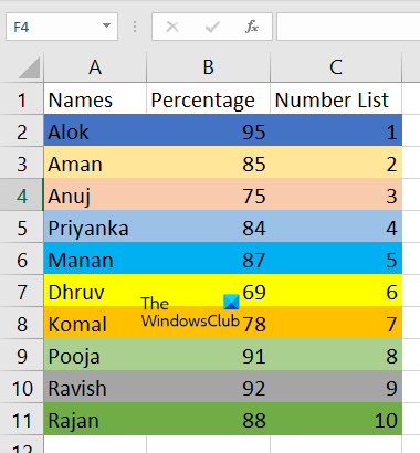
Now, create a new number list in the next adjacent column (see the above screenshot). You have to use this number list to reverse the list in Excel. Excel will treat this number list as a reference to display the desired output.

To do so, follow the steps written below:

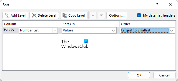
1. Select the entire range of data along with the header.
2. Select the Data tab.
3. Click Sort.
4. The Sort dialog box will appear. In the Sort by drop-down, select the name of the header (in our case, it is Number List).
5. In the Sort On drop-down, select Values.
6. Select Largest to Smallest in the Order drop-down.
7. Click OK.

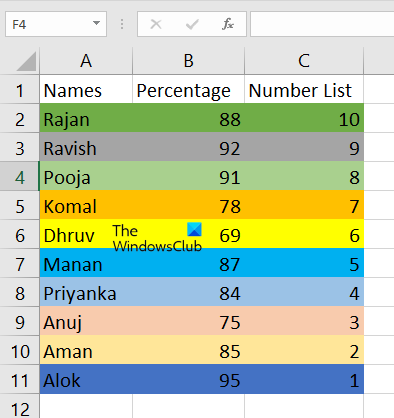
After performing the above steps, the list will be reversed. This is how you can reverse a list in Microsoft Excel by creating a reference number list.

Read: List of best free Excel Add-ins you should be using.

2] How to reverse a list in Excel by using the INDEX function

Let’s see how you can reverse a list in Excel by using the INDEX function. Here, we have a sample list containing the names of the persons and we want to reverse this list.

The format of the formula to reverse a list in Excel by using the INDEX function is as follows:

=INDEX(data range,ROWS(rows range))

Let’s see how to use the above formula. First, select the column in which you want to display the result. Now, copy the header to a cell of that column. We have selected column C and typed the formula to C2.

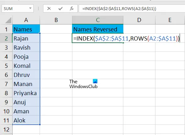
In our case, we want to reverse the list containing the names in the cell range A2 to A11. Hence, the formula is:

=INDEX($A$2:$A$11,ROWS(A2:$A$11))

In the above formula, INDEX($A$2:$A$11) represents the range of the cells containing data to be reversed. The $ sign is used to lock a particular cell in Excel. Here, we have locked the entire range of data. Now, to reverse the list, we have to provide a reference cell to Excel. For this, we have used the ROWS(A2:$A$11) function. In this function, we have locked the A11 cell. Now, Excel will use this cell as a reference cell and treat it as the first cell when it comes to reversing the list. So, in the above formula, only the value without the $ sign will change and the rest of the values will remain locked.

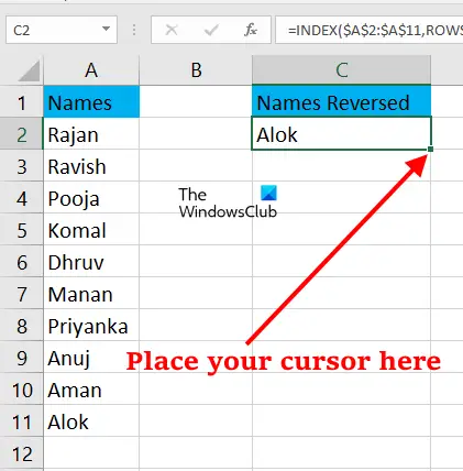
In your case, the address of the cells might differ from ours. Hence, you have to use the formula accordingly. After typing the above formula, press Enter. After that, Excel will display the last name in the targeted cell. As you place your cursor on the bottom right side of the cell, the white cross will turn into a Plus sign. Now, press and hold the left click of your mouse and drag it to the bottom. This action will copy the formula to the other cells.

Above, we have seen how to reverse a single list in Excel using the INDEX function. What if you want to reverse a list having data in multiple columns? In this case, you have to use one more function, COLUMNS. Let’s see how to do that. We have created sample data with three columns.

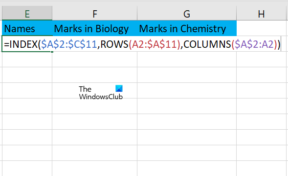
First, select the columns in which you want to display the result. In our case, we have selected columns E, F, and G to display the result. Now, copy the header to the first row of the E, F, and G columns. Select the first cell (after the header) of the first column and type the formula. The formula to reverse a list with data in multiple columns in Excel by using the INDEX function is as follows:

=INDEX($A$2:$C$11,ROWS(A2:$A$11),COLUMNS($A$2:A2))

In the above formula:

• INDEX($A$2:$C$11) represents the entire range of data and the $ sign represents the locked cell. Here, we have locked the entire range of cells containing data.
• ROWS(A2:$A$11) represents the data in the rows from A2 to A11. Here, row A11 is locked as it will be treated as a reference row by Excel. When we copy this formula to other cells, only row A2 will change because it is not locked.
• In the COLUMNS($A$2:A2) function, $A$2 is used as a reference cell. A2 represents column A2. When we copy the formula to the other columns, only the unlocked columns will change.

As described earlier, you need not copy the exact formula and paste it into Excel. If you do so, you may receive an error because your data is not the same as ours. Hence, type the formula according to your data. After typing the formula, press Enter and Excel will display the result in the targeted cell. To display the result, follow any one of the following methods:

• First, copy the formula to all the cells in the first column. After that, copy the formulae from each cell of the first column to the other two columns.
• First, copy the formula to all the cells of the first row. After that, copy the formulae from each cell of the first row to the remaining rows.

Let’s see how to do that. Here, we are using the first method.

Place your cursor on the bottom right side of the first cell. Your cursor will turn from the white cross into a Plus icon. Now, press and hold the left click of your mouse and drag it towards the bottom. This action will copy the formula to all the cells of the first column.

The list in the first column has been reversed. Now, you have to copy the formula in all the cells of the first column to the other columns to reverse the list in respective columns. For this, place your cursor as shown in the above screenshot and drag it towards the right.

 

That’s it. All the lists in the three columns have been reversed. You can also reverse a list in Excel by creating a Macro. We have described this method below.

Read: How to get real-time Currency Exchange Rates in Excel sheet.

3] How to reverse a list in Excel by using a Macro

In Excel, you can create a Macro to run an action or a set of actions as many times as you want. If you use this method, you need not type the formula every time you create a new list in a spreadsheet. Simply, select the range of data and run the Macro. After that, Excel will automatically reverse the list. You can run this Macro to reverse a list with data in a single column and in multiple columns.

First, you have to enable the Developer tab in Excel. After that, select the Developer tab and click Macros. A new window will open. Write the name of your Macro and click Create. In our case, we have given the name ReverseList to Macro. This action will open Microsoft Visual Basic. In the Visual Basic Window, you will see the following text:

Sub ReverseList()
End Sub

The ReverseList is the name of the Macro in the above text.

Now, copy the code written below and paste it into the Visual Basic window.

Dim firstRowNum, lastRowNum, thisRowNum, lowerRowNum, length, count As Integer
Dim showStr As String
Dim thisCell, lowerCell As Range
With Selection
firstRowNum = .Cells(1).Row
lastRowNum = .Cells(.Cells.count).Row
End With
showStr = "Going to reverse rows " & firstRowNum & " through " & lastRowNum
MsgBox showStr

showStr = ""
count = 0
length = (lastRowNum - firstRowNum) / 2
For thisRowNum = firstRowNum To firstRowNum + length Step 1
count = count + 1
lowerRowNum = (lastRowNum - count) + 1
Set thisCell = Cells(thisRowNum, 1)
If thisRowNum <> lowerRowNum Then
thisCell.Select
ActiveCell.EntireRow.Cut
Cells(lowerRowNum, 1).EntireRow.Select
Selection.Insert
ActiveCell.EntireRow.Cut
Cells(thisRowNum, 1).Select
Selection.Insert
End If
showStr = showStr & "Row " & thisRowNum & " swapped with " & lowerRowNum & vbNewLine
Next
MsgBox showStr

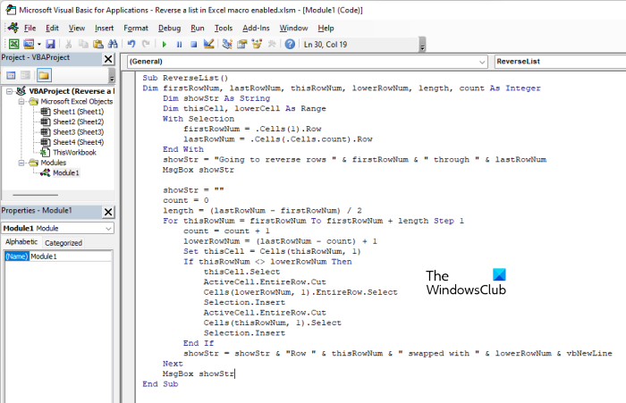
You have to copy the above code between Sub and End Sub in Visual Basic (see the above screenshot). Click on the Save button to save this Macro and close the Visual Basic window.

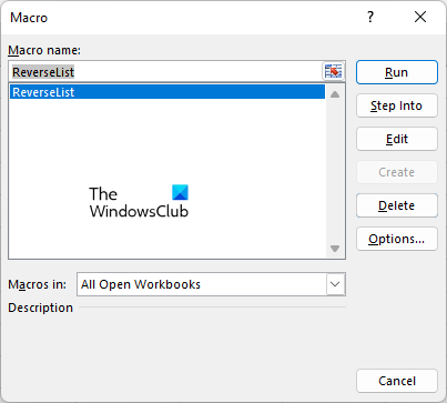
Now, select the entire range of data that you want to reverse, then go to “Developer > Macros.” Select the Macro ReverseList (the name may be different in your case) and click Run. In the confirmation prompt, click OK. After that, Excel will reverse the list.

Hope this helps.

Read: How to Lock and Protect Cells in Excel from editing.

How do you change the direction of a list in Excel?

You can change the direction of a list in Excel by creating a reference number list and then sorting it in decreasing order, by using the INDEX function, and by creating a Macro. Out of these three methods, the first one is the easiest method to reverse a list or change the direction of a list in Excel.

How do I reverse rows and columns in Excel?

You can reverse rows and columns in Excel by creating a reference number list. You have to create this reference list separately for both rows and columns to reverse them in Excel. We have explained how to use the number list to reverse a list in Excel above in this article.

Read next: Microsoft Excel Online tips and tricks to help you get started.