
Excel does not have a built-in feature that literally mixes two colors inside a single cell. However, you can create the appearance of mixed or blended colors using a few practical workarounds. Depending on your goal, you can either blend colors visually or simulate a mixed-color effect based on data. In this guide, we will show you how to mix two colors in Excel on a Windows 11/10 PC.
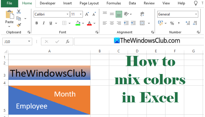
How to mix Colors in Excel
To create a mixed-color effect in Excel on Windows 11/10, use one of the following methods:
- Use Gradient Fill
- Use Shapes
- Use Conditional Formatting
Let us see the above methods in detail.
1] Use Gradient Fill
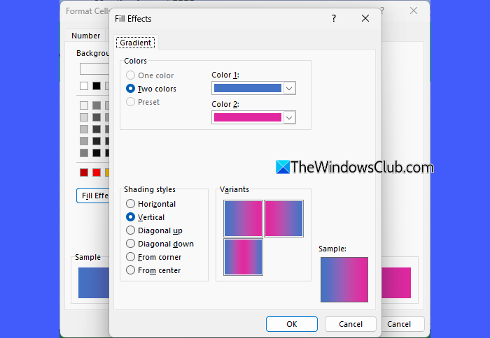
The easiest way to mix two colors in Excel is to use a gradient fill, which blends two or more colors smoothly within a cell.
Open your Excel worksheet and select the cell or range of cells where you’d like to add mixed colors. Right-click and select Format Cells.
In the Format Cells dialog box, go to the Fill tab. Then click Fill Effects.
In the Fill Effects dialog box, make sure Two colors are selected under Colors on the Gradient tab. Click the available dropdowns to select Color 1 and Color 2. You can choose from Theme Colors or Standard Colors.
If you know the exact RGB or Hexadecimal values of the colors you want to mix, click More Colors and enter the values.
Next, select a style under Shading styles. This lets you decide the direction in which you want the colors to appear. You can also select a variant for the selected style under Variants.
Click OK to save the changes. You will now see a smooth transition between the two colors, creating a mixed or blended effect.
2] Use Shapes
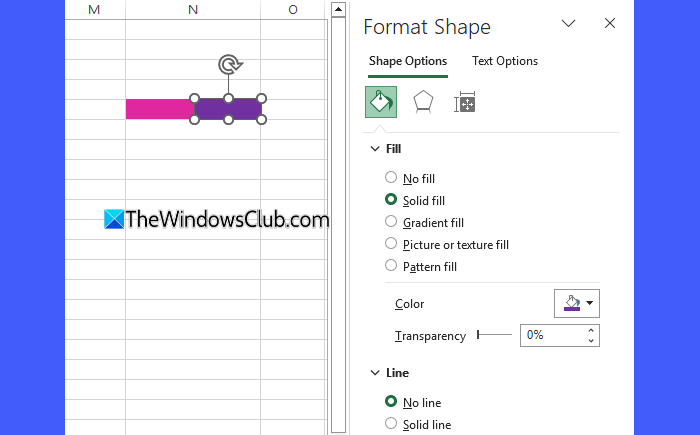
If you want to fill a cell with two solid colors instead of creating a smooth gradient, you can use Shapes. This method allows you to divide a cell vertically, horizontally, or diagonally and apply different colors to each section.
Open your Excel worksheet and select the cell where you want to create the two-color effect. Go to the Insert tab. Click Shapes, and select Rectangle.
Draw the rectangle over one half of the cell. Right-click the shape and select Format Shape.
The Format Shape pane will open on the right side. Under Fill, select Solid fill, then use the Color drop-down to select the first color. Under Line, select No line to remove the outline around the shape.
Next, copy the shape and place the copy over the other half of the cell. Then follow the same steps to select a different fill color for the second shape. Adjust the size and position of both shapes so that they fit neatly within the cell.
You can also create a diagonal two-color effect by using shapes such as Triangles. This can be useful when creating tables where you want to place two headers in a single cell and visually separate them with a diagonal line. You can then apply different colors to the two headers to make them easier to distinguish.
Note: Shapes are floating objects and are not part of the cell formatting. If you change the row height or column width, you may need to resize or reposition the shapes.
3] Use Conditional Formatting
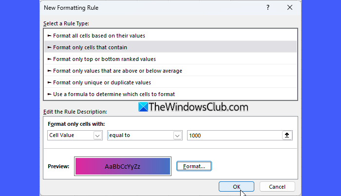
You can also use Conditional Formatting to apply a gradient fill to cells that meet a specific condition. For example, if you want to highlight cells that contain a particular value, you can create a rule and then apply a gradient fill to the matching cells.
Select the cell or range of cells where you want to apply the formatting. Go to Home > Conditional Formatting > New Rule.
In the New Formatting Rule dialog box, select a rule that matches your requirement. For example, select Format only cells that contain, then under Edit the Rule Description, use the available dropdowns/options to create the rule.
Next, click Format. In the Format Cells dialog box, go to the Fill tab and click Fill Effects. Then follow the same steps explained in the first method to select desired colors, shading style, and variant.
Click OK to save the rule. Excel will now apply the selected gradient fill to cells that meet the specified condition.
You can create additional Conditional Formatting rules if you want to apply different gradient fills to cells with different values or that meet different conditions.
That’s all! I hope you find this useful.
Read: Most useful Excel Tips and Tricks for beginners.
How to split a cell color in Excel?
Excel does not provide a direct option to split a cell into two independently colored sections. However, you can create a similar effect using Shapes by placing two colored rectangles or triangles over the cell. Alternatively, you can use a gradient fill to create a smooth transition between two colors within the cell.
Can you have two colors in an Excel cell?
Yes, you can create a two-color effect in an Excel cell using a gradient fill. Select the cell, go to Format Cells > Fill > Fill Effects, select Two colors, and choose the colors and shading style you want.
Read Next: How to play Video and Audio in Excel.
