Budgeting is a tough task. It needs a lot of thinking, the right tool, and a simple-to-understand dashboard. In the time when even a mediocre app is sold at a subscription to track finances, we can build a simple personal finance tracker on Google Sheets. All it takes is a Google account and implementation of our tips. Learn how to automate budgeting on Google Sheets.
How to automate Budget on Google Sheets
It takes multiple steps to create a Google Sheets sheet to automate the monthly budget and track income and expenses without calculation errors. Follow the steps below to end up with a sheet that takes your numbers as input and gives you a detailed overview of your finances.
- Create sheets for Income & Expenses, Categories, and a Dashboard
- Organize columns to record transactions
- Make Categories for every income and spend
- Summarize your finances automatically
- Understand your budget
Let’s get into the details and prepare a Google Sheets sheet we can reuse every month to automate the budget for free.
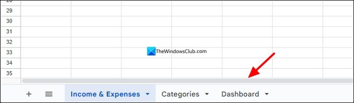
Open a web browser on your PC and head to sheets.google.com and create a new spreadsheet. Rename the default Sheet1 as Income & Expenses. Add another sheet by clicking the + icon and name it Categories. Add a third sheet and name it Dashboard.
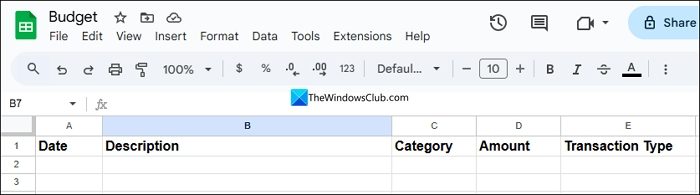
Click on the Income & Expenses sheet and create columns for Date, Description, Category, Amount, and Transaction Type, where you can enter the dates of each income and spends, write about it, enter the amount, and set it as income or expense in the Transaction type column.
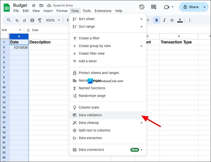
After creating the columns successfully, ensure they support the input type. The date column must accept dates in its format, Amount column must support your currency. To set the correct date format, select the Date column and click Data on the menu bar. Select Data validation.
It opens Data validation rules on the sidebar. Click Add rule.
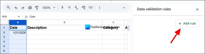
You need to apply the column range from A2 because A1 is occupied by the Date as a title. Since you have selected the entire column, the range is set from A1. Change it by replacing ‘1’ with ‘2’ in the Apply to range section. Click the dropdown under Criteria and select is valid date. Then, click Done to save the changes.
It will make sure you only enter the date in the Date column. We cannot set the data validation rules of the Amount column. We can enter the amount details with your currency symbol, like $.

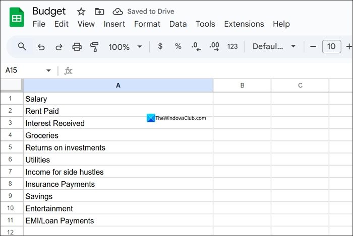
Now move to the Categories sheet and enter the income categories, such as Salary, Freelancing, etc. Then, enter your expenses like Groceries, Bills, Staples, Rent, etc. Make sure you enter every category you receive and spend your money on. It would make your sheet look better in the dashboard, and give you a clear idea of what is taking up most of your budget. You need to enter the categories in the same column, one after the other, as shown in the image below.
In the Income & Expenses sheet, we have a Categories column. When we enter amounts, we have to select the Category there. We need to connect the categories we listed on the Categories sheet to the Category column in the Income & Expenses sheet.
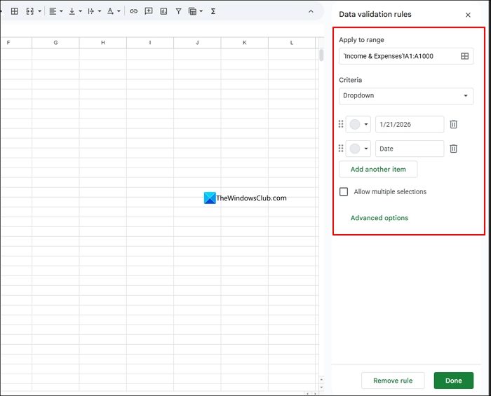
Go to the Income & Expenses sheet and select the Category column and click Data on the menu, and select Data validation. On the Data validation rules that appear on the sidebar, click +Add rule.
Now, select the range from the C2 cell, as C1 contains the title. Click the dropdown under Criteria and select Dropdown (from a range). It shows a box below it to select a range. Click on the box. It opens the Select a data range pop-up. Click the Categories sheet and select all the listed categories, and click OK. Then, click Done to save the changes and apply the rule to the Category column.

Every cell in the Category column will now have a dropdown to select a category. In the future, if you want to add a new category, just add it to the Categories sheet and update the Data validation rules to reflect the change by adding cells for the newly added category.
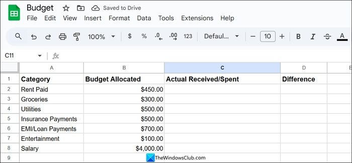
Go to the Dashboard sheet and add Category, Budget Allocated, Actual Received/Spent, and Difference columns, and fill them. Enter the category that you have already listed in the Categories sheet, then enter their budget allocation against each of them. Create columns of Actual Received/Spent and Difference, which we will calculate in the next steps.
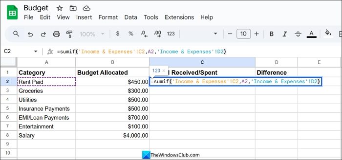
We will now use the SUMIF function to summarize our budget in the Dashboard sheet. The SUMIF function can seem scary at first, but once we understand its syntax, there is no going back. Without the SUMIF function, there is no dashboard or this budgeting sheet. The following is the syntax of the SUMIF function on Google Sheets.
=SUMIF(range, criterion, [sum-range])
To explain the SUMIF function simply, it contains three elements, as shown in the syntax. The first element is range. It is the range of cells that you want to test against the second element, the criterion. The criterion in the syntax is the condition that determines which cells to add, as needed. The third element in the syntax, sum_range, sums the actual cells.
Now, it is time to apply the SUMIF function to our budget sheet and summarize the budget. So, for the first input, we have Rent Paid. Click on the cell against it under the Amount Received/Spent column.
Type SUMIF( and click on the Income & Expenses sheet and select Rent Paid entry in the Category and type , to denote that the first element is completed. Then, come to the Dashboard sheet and select Rent Paid under the category, A2, in the sheet shown below, and type a comma to complete it. Then, go to the Income & Expenses sheet and select the Amount against the category. Complete the syntax by closing the bracket and pressing Enter.
Then, drag the formula to the cells below to auto apply it. It is time to calculate the difference. It is a simple subtraction. Click on the cell under Difference and type B2-C2 and press Enter. Drag the same to apply to the rest of the cells.
It is time for the final step, where we calculate Net income. Net income is the amount remaining after deducting total expenses from total income. We will use the SUMIF function again to calculate it. It has only two categories: Income or Expenses. So, the formula is simple. To calculate Total income, use the following function.
=SUMIF('Income & Expenses'!E:E, Income, 'Income & Expenses'!D:D)
Similarly, to calculate Total Expenses in the Sheet, use the following function.
=SUMIF('Income & Expenses'!E:E, Expenses, 'Income & Expenses'!D:D)
To find out Net income, just subtract Total Expenses from Total Income.
Read: How to create an automated Budget in Excel
Is it safe to use Google Sheets for budgeting?
It is very safe to use Google Sheets for budgeting, as it is saved to your Google account, and no one can access it without your Google account. You also do not need to pay any subscription fee; you can use it for free for a lifetime and access it anywhere on any device.
Does Google have a budgeting tool?
Google provides budget templates in Google Sheets. If you want a customized sheet that suits your needs, you can create one yourself, as we have shown. It takes some time to create your first sheet, but once you get the logic and syntax, there is no going back.
Also read: Free Personal Finance & Business Accounting Software for PC.