Dropdowns are useful features that simplify data entry and enforce data validations in spreadsheet software. Creating a dropdown list is easy. And you might have done that already in Excel. But did you know, you can also assign a background color to your dropdown list items? A colored dropdown makes your data easier to read and makes user selections easier to identify. In this post, we will show how to create a dropdown list in Microsoft Excel. We will also show you how to make a colored and nested drop-down list.

If you use Microsoft Excel as your preferred analytic tool, you might already be familiar with the concept called conditional formatting. Conditional formatting, as the name suggests, is used to format the content of a cell based on a certain condition. For example, you may use conditional formatting to highlight duplicate cell values. Similarly, you may use conditional formatting to assign colors to items in a drop-down list.
How to create a drop-down list in Excel
To create a drop-down list in Excel, follow these steps-
- Select a cell where you want to show the drop-down menu.
- Go to Data > Data Validation.
- Select the List from the Allow menu.
- Write down your options in the Source box.
- Save your change.
To get started, you need to select a cell in your spreadsheet where you want to show the drop-down list. After that, switch from the Home tab to the Data tab. In the Data Tools section, click the Data Validation button, and select the same option again.

Now, expand the Allow drop-down list, and select List. Then, you need to write down all the options one after one. If you want to display AA, BB, and CC as the examples, you need to write them like this-
AA,BB,CC
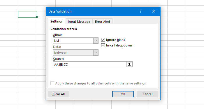
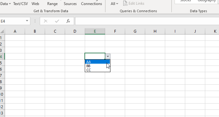
No matter how many options you want to provide, you need to separate them by a comma. After doing that, click the OK button. Now, you should find a drop-down list like this-
You can add an error message as well. It appears when users try to enter a different value other than the given options. For that, switch to the Error Alert tab, and write down your message. Follow this tutorial to add error messages in Excel.
Read: How to create a drop-down list in Google Sheets with color.
How to create a dropdown list in Excel with color

To create a color-coded dropdown list in Microsoft Excel, you first need to create a dropdown list and then you can move ahead to add colors to the list items.

Let us say we have a sample spreadsheet as shown in the above image wherein we have a list of tasks that needs to be marked as ‘New’, ‘In Progress’, ‘Done’, or ‘Not Done’. To take user input, we will first create the dropdown list as follows:
- Select cell B2.
- Go to the Data tab.
- Select Data Validation from the Data Tools section.
- Select List from the Allow dropdown.
- Type ‘New,In Progress,Done,Not Done’ in the Source field.
- Click on the OK button.

The above steps will create a dropdown list next to the first task in the spreadsheet. Next, we will add colors to the dropdown list items as follows:
- Select cell B2.
- Go to the Home tab.
- Click on Conditional Formatting in the Styles section.
- Select New Rule from the dropdown that appears.

- Select Format only cells that contain under Select a Rule Type.
- Under Format only cells with, select (and type) Specific Text > containing > ‘New’, where ‘New’ refers to the item in the list.
- Click on the Format button.

- In the Format Cells window, switch to the Fill tab.
- Select the color that should be associated with the dropdown list item ‘New’. In this example, we are applying a shade of yellow to the new tasks assigned.
- Click on the Ok button.

- Click on the Ok button again in the next window. So far, we have associated color with the list item ‘New’.
- Repeat the process (steps 1 to 11) for other list items – ‘In Progress’, ‘Done’, and ‘Not Done’, while applying a different color to each of them. We have applied a shade of blue, a shade of green, and a shade of red to these items in this example.
- Go to Home > Conditional Formatting > Manage Rules to open the Conditional Formatting Rules Manager.

- Preview and verify all the rules that you’ve applied to the dropdown list items and click on OK. Now you have a color-coded dropdown list in cell B2.
- Take the cursor to the bottom-right corner of cell B2.
- As the cursor turns into a plus (+) symbol, click and drag the cursor till cell B6. This action will copy the cell content and the corresponding formatting rules of cell B2 to the cell range B3:B6 (where we need to have the dropdown list).
Read: How to add a Tooltip in Excel and Google Sheets.
How to create a nested drop-down list in Excel
If you want to obtain data from some existing drop-down menus or cells and display options accordingly in a different cell, here is what you can do.
You need to open the same Data Validation window and select List in the Allow menu. This time, you need to enter a range in the Source box like this-
=$A$1:$A$5
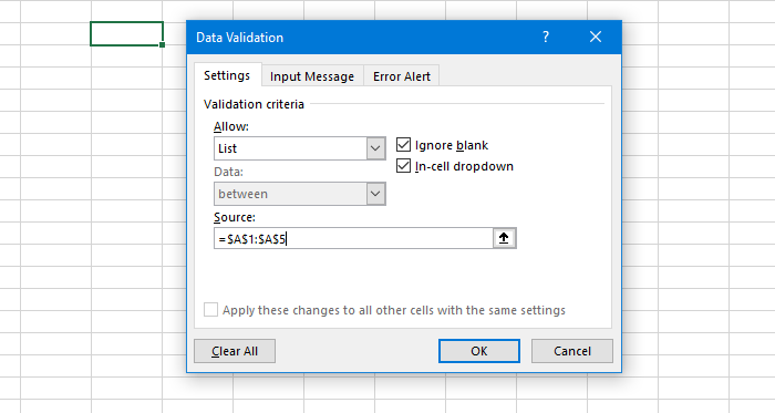
According to this range, the new drop-down list will show the same options that are written in the A1 to A5 cells.
Read: How to connect Google Sheets with Microsoft Excel.
How do I change the color of a selected value in a dropdown?
In Microsoft Excel, select the cell where the dropdown is placed. Go to Home > Conditional Formatting > Manage Rules. Double-click on the desired color. Click on the Format button in the next window. Choose a different color and click on OK. In Google Sheets, select the dropdown and click on the edit (pencil) button at the bottom of the item list. Select the desired color using the color options available in the right panel and click on the Done button.
Related reads: