How to create a drop-down list in Excel and Google Sheets

If you are creating an interactive spreadsheet, you may need a drop-down list so that users can choose between options. For that, you can follow this tutorial to create a drop-down list in Microsoft Excel or Google Sheets. You can create a single as well as a nested drop-down menu with the help of this guide.

Like various programming languages, it is possible to include the if-else statement in an Excel spreadsheet as well. Let’s assume that you are creating a spreadsheet for people who should select different options according to various criteria. At such a moment, it is wise to use a drop-down list so that you can provide more than one choice to the people.

How to create a drop-down list in Excel

To create a drop-down list in Excel, follow these steps-

1. Select a cell where you want to show the drop-down menu.
2. Go to Data > Data Validation.
3. Select the List from the Allow menu.
4. Write down your options in the Source box.
5. Save your change.

To get started, you need to select a cell in your spreadsheet where you want to show the drop-down list. After that, switch from the Home tab to the Data tab. In the Data Tools section, click the Data Validation button, and select the same option again.

Now, expand the Allow drop-down list, and select List. Then, you need to write down all the options one after one. If you want to display AA, BB, and CC as the examples, you need to write them like this-

AA,BB,CC

No matter how many options you want to provide, you need to separate them by a comma. After going that, click the OK button. Now, you should find a drop-down list like this-

You can add an error message as well. It appears when users try to enter a different value other than the given options. For that, switch to the Error Alert tab, and write down your message. Follow this tutorial to add error messages in Excel.

How to create a nested drop-down list in Excel

If you want to obtain data from some existing drop-down menus or cells and display options accordingly in a different cell, here is what you can do.

You need to open the same Data Validation window and select List in the Allow menu. This time, you need to enter a range in the Source box like this-

=$A$1:$A$5

According to this range, the new drop-down list will show the same options that are written in the A1 to A5 cells.

How to create a drop-down list in Google Sheets

To create a drop-down list in Google Sheets, follow these steps-

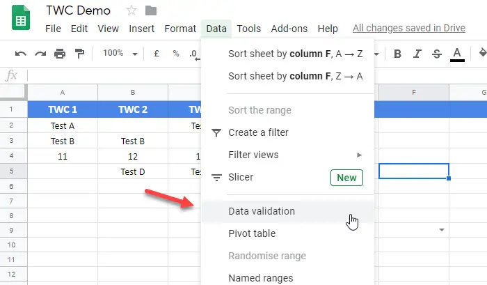
1. Select a cell and go to Data > Data validation.
2. Select the List of items.
3. Write down your items or options.
4. Save your change.

At first, select a cell in a spreadsheet and click the Data from the top navigation bar. After that, select the Data validation option from the list.

Now, expand the Criteria drop-down menu, and select List of items. Next, you need to write down all the options or items in the empty box.

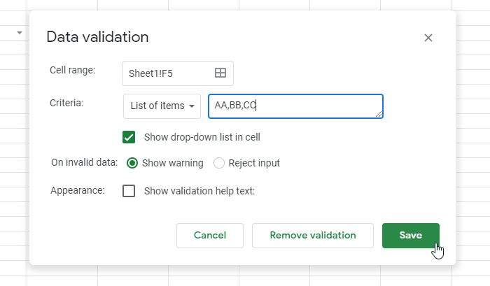
At last, click the Save button to show the drop-down list in a cell.

Like Excel, Google Sheets shows a warning or error message for entering invalid data. By default, it shows a warning message and allows users to write custom text. If you want to prevent users from entering invalid data, you need to choose the Reject input option in the Data validation window.

How to create a nested drop-down list in Google Sheets

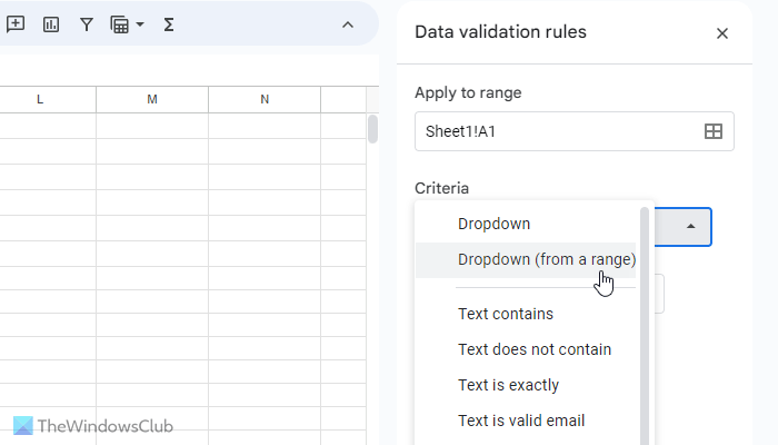
It is almost the same as Excel, but the name of the option is different. You need to select the List from a range option from the Criteria list and enter a range according to your needs. You can enter a field like this-

=$A$1:$A$5

It will show all the texts from A1 to A5 cells in this drop-down list.

That’s it! Hope it will help you.