
Conditional formatting is a powerful tool for visually highlighting data, but it can be frustrating when the rules seem to apply to some cells but not others. This issue often stems from incorrect range references, relative vs absolute addressing, or data type mismatches. In this post, we will see what to do if Conditional formatting is not applying to all cells in Excel or Google Sheets.
Fix Conditional formatting not applying to all cells in Excel or Google Sheets
In Excel, common causes include using relative references in formulas (so the rule shifts unexpectedly), mismatched data types (e.g., numbers stored as text), or having multiple overlapping conditional formatting rules where one overrides another. In Google Sheets, reasons often include the Apply to range field not covering all intended cells, custom formulas referencing fixed cells incorrectly, or blank cells being ignored by certain rule types, such as blanks or text contains.
If Conditional formatting is not applying to all cells in Excel or Google Sheets, follow the solutions mentioned below.
- Verify and expand the Applies to Range
- Use Absolute References in Custom Formulas
- Convert Number Stored as Text to Real Numbers
- Remove or Reorder Conflicting Rules
Let us talk about them in detail.
1] Verify and expand the Applies to Range
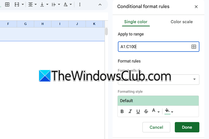
Conditional formatting only affects the range explicitly specified. If you add new rows or columns outside that range, they won’t inherit the rule. Extending the range ensures every target cell is covered. To do the same, follow the steps below.
Excel
- Select any call with the conditional formatting.
- Now, go to Home > Conditional Formatting > Manage Rules.
- In the dialog, select the rule and click on Edit Rule.
- IN the Applies to box, enter the full range (e.g., =$A$1:$C$100 instead of =$A$1:$A$10).
- Click OK > Apply.
Sheets
- Select the cell range where formatting should apply.
- Now, click Format > Conditional formatting.
- In the sidebar, check Apply to range.
- Edit it to include all cells (e.g., A1:C100).
- Click Done.
Finally, check if the issue persists.
2] Use Absolute References in Custom Formulas
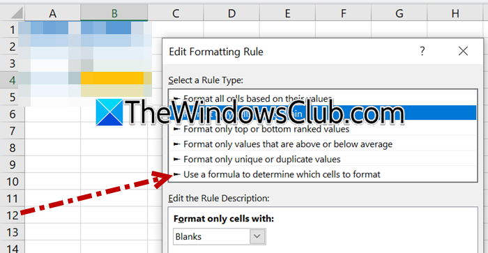
When you write a custom formula (e.g., =A1>10), Excel and Sheets interpret it relative to the top-left cell of the applied range. Without dollar signs, the reference shifts for each cell, breaking the intended logic. Absolute references keep the comparison fixed to a specific cell or column. Follow the steps mentioned below to do the same.
Excel
- Manage rules as above, go to Edit Rule > Use a formula to determine which cells to format.
- Change the formula to use absolute references where needed, so, like =$A$1>10 to always look at cell A1.
- Ensure the Applies to range is correct and click on OK > Apply.
Sheets
- Open the Conditional formatting sidebar.
- Under Format cells if, choose Custom formula is.
- Enter the formula with absolute references (eg,. =$A$1>10).
- Confirm the Apply to range includes all target cells.
- Click Done.
Now, see if the formatting applies to all cells.
3] Convert Numbers Stored as Text to Real Numbers
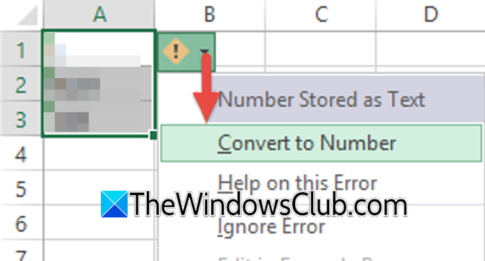
Many conditional formatting rules (e.g., greater than, between, or color scales) only work on numeric values. If some cells contain numbers stored as text (often indicated by a green triangle in Excel or left alignment in Sheets), the rule skips them. Converting them to true numbers makes the rule apply uniformly.
Excel
- Select the problematic column/range.
- Look for a small yellow diamond with an exclamation mark.
- Click on it and select Convert to Number. Or use Text to Columns > Data > Text to Columns > Finish (no changes needed).
- Reapply or check Conditional formatting.
Sheets
- Select the range with numbers stored as text.
- Click Data > Data cleanup > Convert to number. Or use a helper column: =VALUE (A1), then copy-paste values back.
- Verify the conditional formatting now applies to all cells.
Finally, check if the issue persists.
4] Remove or Reorder Conflicting Rules
Both Excel and Sheets evaluate multiple rules in order. If two rules apply to the same cell, the first rule’s formatting can be overridden by a later rule with Stop if True (Excel) or simple priority (Sheets). Removing duplicates and reordering ensures your intended rule takes precedence.
Excel
- Go to Home > Conditional Formatting > Manage Rules.
- In the list, look for duplicate or overlapping rules for the same range.
- Select a lower-priority rule and click Delete or use the Move Up/Down arrows to reorder.
- Check the Stop if True box for the rule you want to dominate.
- Click Apply.
Sheets
- Go to Format > Conditional formatting.
- In the sidebar, you will see all the rules listed for that sheet.
- Over a rule and click the trash can to delete duplicates.
- Drag rules (three‑dot icon) to change evaluation order; the top rule runs first, but Sheets applies all rules; delete contradictory ones.
- Click Done.
Now, you need to check if the issue persists.
That’s it!
Read: How to Create a Calendar in Google Sheets
Why is conditional formatting not applying to all cells in Google Sheets?
This typically happens when the Apply to range field doesn’t cover your entire target area, often because you added rows after setting the rule, or entered A1:A10 instead of A1:A100. Another cause is using a custom formula with relative references (e.g., =A1>10) that shifts per cell, or having conflicting rules where one overrides another. Data type mismatches, like numbers stored as text, can also prevent full application.
Read: How to Highlight Duplicates in Google Sheets?
Can you apply conditional formatting to an entire sheet?
Yes, in Google Sheets, delete any existing range and type A1:Z or A1:1000, or click the blank rectangle above row 1 to select all cells. In Excel, click the triangle at the top‑left of the grid, then set your rule; the Applies to field will show =$1:$1048576.
Also Read: Highlight Rows with Dates using Conditional Formatting in Excel
