
Timelines are essential for planning, tracking, and communicating time-based data. They are visual tools that display the chronological sequence of milestones, deadlines, and other significant past or future events on a time scale, making it easier to understand the flow and progress of projects over time. In this post, we’ll walk you through several ways to create a timeline in Microsoft Excel on a Windows 11/10 PC.
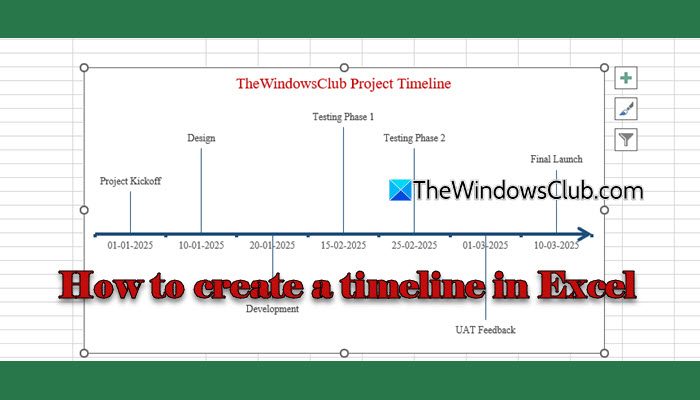
How do I create a Timetable in Excel?
If you’re working in Excel, you don’t need to rely on any external software to build a professional-looking timeline. From using basic charts and bar graphs to leveraging SmartArt and templates, Excel offers several built-in features that let you create effective and customizable timelines with ease.
How to create a Timeline in Excel
In this guide, we will show you the following ways to create a timeline in Excel:
- Using Column Chart
- Using SmartArt
- Using Templates
Let us see this in detail.
1] Create a timeline using Column Chart
A Column Chart can be used to create the most common form of a timeline in Excel, which consists of a horizontal layout with a time-based X-axis and events or milestones plotted along it.
To create a basic timeline using a Column Chart, you’ll need three columns of data:
- Unit of Time: This can be a date, month, or year that marks when the event occurs.
- Event Name: A short label or description of the milestone or event.
- Event Height: A numeric value used to plot the height and direction of the column. You may use positive and negative numbers to alternate the columns up and down along the X-axis. This improves readability and prevents overlapping labels.
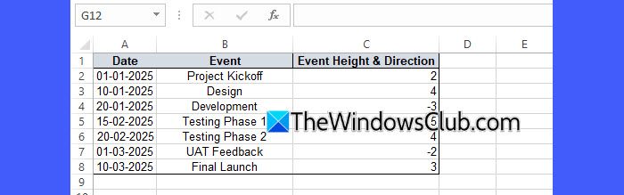
Suppose we have the following data, wherein Column A contains the dates, Column B lists the project events, and Column C holds numeric values that determine both the height and direction of each event on the timeline, as shown in the image below:
To create a timeline for this data, follow these steps:
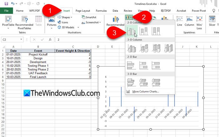
Select columns A and C, excluding the headers. Go to the Insert tab in the top ribbon. Click the Insert Column or Bar Chart dropdown (under the Charts section) and select Clustered Column.
Click the Chart Elements button (the plus symbol that appears when the chart is selected). Click the arrow next to Data Labels (appears on hover-over) and select More Options. A Format Data Labels panel will appear on the right side.
In the panel, uncheck the Value option and check the Value From Cells option. Select the cells of the Event column and click OK in the Data Label Range dialogue. This replaces the default numeric values (which would normally show as data labels) with the text from your Event column.
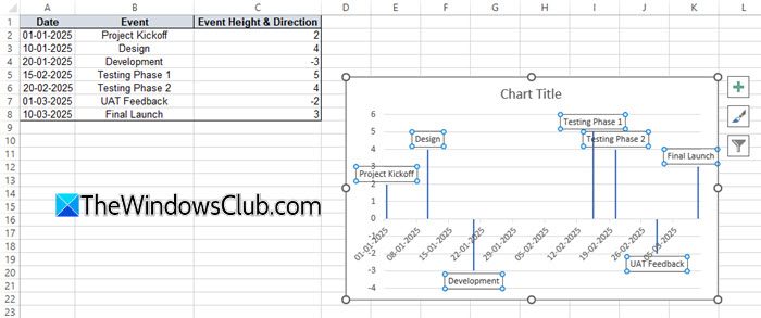
Click the Data Series and go to the Format tab. Select Shape Fill > No Fill. Again, click the Chart Elements menu, then click the arrow next to Error Bars and select More Options. In the Format Error Bars panel, select Minus for Direction, No Cap for End Style, and Percentage for Error Amount. Set the Percentage to 100%.
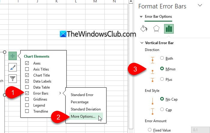
By hiding the column’s fill and adding formatted Error Bars, you replace the thick bars with thin vertical lines that neatly connect each event marker to the timeline axis.
The timeline is ready, but we’ll format it a bit to give it a clean look.
Again, click the Chart Elements menu, click the arrow next to Axes, and uncheck Primary Vertical. Also, uncheck the Gridlines option. Then select the chart outline, go to Format > Shape Outline > No Outline.
Next, select the horizontal axis and go to the Format tab. Click the Shape Outline dropdown and select a brighter color for the axis. Also, change the Weight to 3 pt and Arrows to Arrow Style 2. Next, click the error bars and change their colors to.

You can also adjust the distance of the events from the timeline by updating the values in the Event Height column.
Finally, give a suitable title to your timeline chart, and you’re done!

2] Create a timeline using SmartArt
SmartArt provides a quick and easy way to create a timeline in Excel without having to set up or plot data with chart tools. Instead, you insert a SmartArt graphic and then manually type your event names and dates into the timeline shapes.
For SmartArt, you only need two pieces of information: Date (unit of time) and Event Name (milestone description). You do not need the height/direction values, because SmartArt does not plot points on axes.
Suppose we have the same sample data as above. To create a timeline from that data using SmartArt, follow these steps:
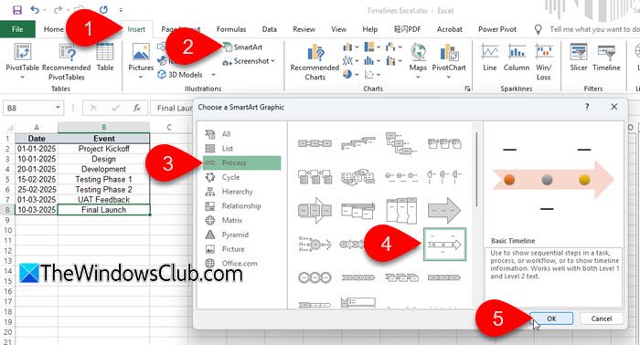
Go to the Insert tab in the top ribbon. In the Illustrations group, click SmartArt.
In the Choose a SmartArt Graphic dialog box, select Process from the left pane. You will see various process layouts. Scroll down and select Basic Timeline (or any timeline style you prefer), then click OK.
A SmartArt graphic will appear on your sheet. Click the small arrow on the left edge of the SmartArt to open the Text Pane. Click inside each placeholder (Text) to edit it and add your milestone. Press Enter after an item to create another milestone, and press Tab to create a second‑level bullet where you can add the date or additional details for that milestone.
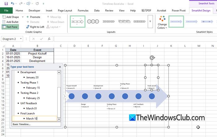
Next, format your timeline to match your style. Click the SmartArt graphic, go to the SmartArt Design tab, and choose a style or color theme from the gallery. You can also use the Format tab to change shapes, outlines, or effects for a cleaner look.
Finally, resize and position your timeline as needed, give it a clear title, and your SmartArt timeline is ready to use!
3] Create a timeline using Templates
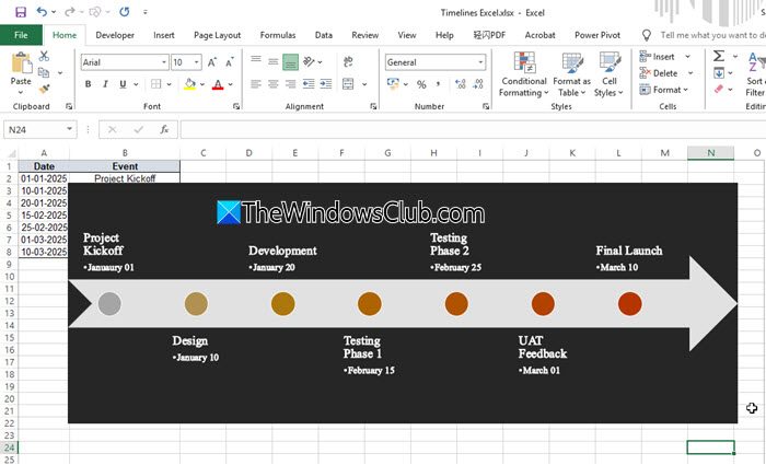
Another quick way to build a timeline in Excel is by using pre‑built templates. Microsoft and many other sources offer ready‑made Excel timeline templates that already include formatted charts, sample data, and styles. You only need to replace the sample information with your project dates and milestones. This is a great option if you want a professional‑looking timeline quickly, without manually creating charts or formatting them yourself.
To use this method, simply open Excel and search for timeline templates from the File > New screen (or download a template from trusted sources like Microsoft Office Templates).
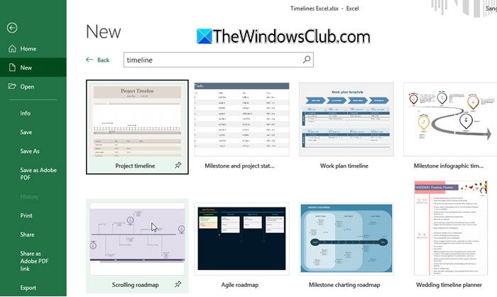
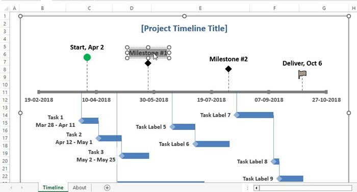
Select the desired template and click Create. This will open the template as a new Excel file. Double‑click any text in the template to change it. Click objects to select them. Use the Format tab to edit a shape’s color, outline, and text style.
That’s all! I hope you find this useful.
Read: How to create a Timeline in PowerPoint.
How do I create a Gantt timeline in Excel?
To create a Gantt timeline in Excel, set up a table with columns for Task, Start Date, and Duration. Then select the Start Date and Duration columns, excluding headers. Go to the Insert tab, and select Bar Chart > Stacked Bar. In the chart, add Task names to the vertical axis. Then adjust the axis, reorder tasks if needed, and style the bars to clearly show your project schedule.
Read Next: Microsoft Excel time-saving tricks to work faster.
