In Microsoft Excel, if a cell contains a formula that results in an error, a triangle appears in the top-left corner of the cell. The triangle is an error indicator. The default is green but you can change to any other that you like.
How to change the Color of an Error Indicator in Excel
Follow the steps below to change the color of an error indicator in Microsoft Excel:
- Click the File tab on the menu bar.
- Click Options on the backstage view.
- Excel Options.
- An Excel Options dialog box will open.
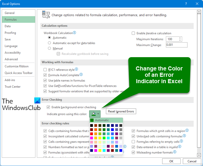
- Click the Formulas tab on the left pane.
- Under the Error Checking section, click the list box for ‘ Indicate errors using this color’ and choose a color from the list.
- Click Ok.
- The error indicator in the cell turns red.
Click the File tab on the menu bar.
Click Options on the backstage view.
An Excel Options dialog box will open.
Click the Formulas tab on the left pane.

Under the Error Checking section, click the list box for ‘ Indicate errors using this color’ and choose a color from the list.
Click Ok.
The error indicator in the cell turns red.
We hope this tutorial helps you understand how to change the color of an error indicator in Excel; if you have questions about the tutorial, let us know in the comments.
Read: How to use Goal Seek in Excel?
How do you identify errors?
In Microsoft Excel, you do not have to identify an error; Excel will do that for you. You will see an error pop up in your cell, with a green triangle at the top left. In Microsoft Excel, a handful of errors can appear in your cells, such as Ref, null, Num, Value, etc.
Why do spreadsheets have errors?
Like most programs, errors can be triggered in Microsoft Word. Errors can occur in Excel due to users typing incorrect formula references, accidentally deleting an important cell or row, and more.