If you want to count blank or empty cells in Excel and Google Sheets, here are the exact formulas you need to use. There are three ways to count blank or empty cells in any spreadsheet and here we have enlisted all of them so that you can use them as per your requirements.
Microsoft Excel and Google Sheets support countless functions so that users can perform various jobs. There are some functions called COUNTBLANK, COUNTIF, SUMPRODUCT, etc. that will help you to count blank or empty cells. Sometimes, you may need to count all empty cells in a spreadsheet. If it has two or three columns and ten or twenty rows, you can calculate them manually. However, the problem starts when you go to count the empty cells of a large spreadsheet. That is when you can use this trick to get the exact number of blank cells in Google Sheets or Excel.
Count blank or empty cells in Excel or Google Sheets
To count blank or empty cells in Excel or Google Sheets, follow these steps:
- Open the spreadsheet in Google Sheets or Excel.
- Choose the column.
- Click on a cell where you want to show the number.
- Use COUNTBLANK, COUNTIF or SUMPRODUCT function.
To learn more about these steps and functions, continue reading.
First, you need to open the spreadsheet in Google Sheets or Microsoft Excel. Now you should note down the columns/rows for which you want to find the number of empty cells. It can be one or multiple columns, and it depends on your requirements.
After that, click on an empty cell in your spreadsheet where you want to display the number. Then, enter a function like this-
=COUNTBLANK(A2:D5)
This COUNTBLANK function counts empty cells between A2 and D5. You can change the column/row number as per your needs.

There is another function that does the same job as COUNTBLANK. It is called COUNTIF. This function is handy when users need to count cells containing a specific word, digit or symbol. However, you can use the same function to count the empty cells in Google Sheets as well as the Microsoft Excel spreadsheet.
To use this method, you need to open a spreadsheet, select a cell, and enter this function-
=COUNTIF(A2:D5,"")
You need to change the range according to your requirements. The COUNTIF function requires a value between inverted commas. As you are going to find blank cells, there is no need to enter any value or text.
The main difference between COUNTBLANK and COUNTIF functions is that the first one is mainly used to find blank cells whereas the latter one is used to find almost anything.
The third function is SUMPRODUCT. Although it is quite different from other functions because of its characteristics, you will get the job done with the help of the SUMPRODUCT function.
As usual, you need to select a cell where you want to display the number and enter this function-
=SUMPRODUCT(--(A2:D5=""))
You need to change the range before entering this function and do not write anything between the inverted commas.
Hope this tutorial helps you.
Read: How to remove Blank Cells from Microsoft Excel spreadsheet
How do you count empty cells in a sheet?
There are three functions you can use to count empty cells in a sheet. They are: COUNTBLANK, COUNTIF, and SUMPRODUCT. Although each formula works in a different way, you can find the result without any error if you can enter the cell range correctly. The easiest way to count blank or empty cells in a spreadsheet is by using the COUNTBLANK function. Enter the function like this: =COUNTBLANK(A2:D5) where A2/D5 is the cell range.
How do I check for blanks in Excel?
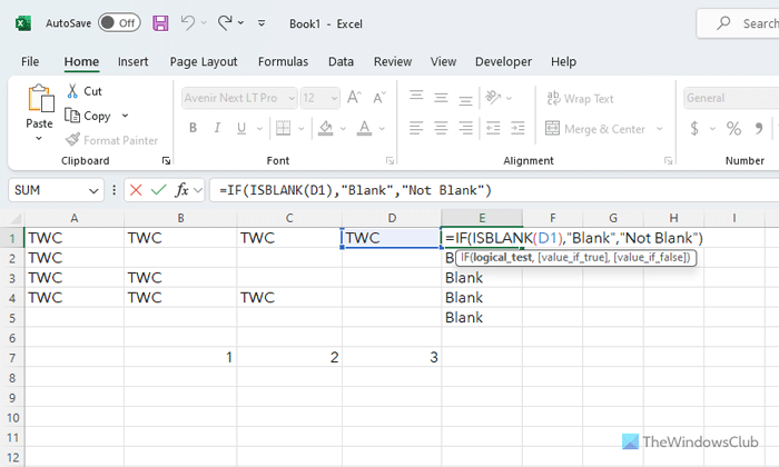
To check for blanks in Excel, you can use a simple function called ISBLANK with IF. In simple terms, the IF function is used to check whether a certain condition matches or not. On the other hand, ISBLANK denotes where it says – it finds the blank cell. In order to use this formula, you need to nest them like this: =IF(ISBLANK(A1),”Blank”,”Not Blank”) where A1 is the cell to find whether it is blank or not. for obvious reasons, you need to apply this formula in a different column.
Read: How to count Nonblank Cells in Excel